Author: Jade Mitchell and Sushil B. Tamrakar

General overview

Inactivation of vegetative microorganisms, there are several types of survival curves that described the inactivation rates and patterns(Xiong, Xie et al. 1999). The most commonly used mathematical linear model is first order exponential model. However, in many cases linear model alone cannot describe the prevailing pattern. There are several nonlinear models described by various investigators to fit the data (Coroller, Leguerinel et al. 2006). Seven different models described in various studies have been shown in Table 1.(Peleg and Cole 1998; Juneja, Eblen et al. 2001; Valdramidis, Bernaerts et al. 2005; Juneja, Huang et al. 2006).

The data from each treatment was fitted to a best-fit curve using an unpublished mathematical model fitting tool in Microsoft® Excel (Microsoft® Inc., Redmond, Washington) by Patrick Gurian at Drexel University and modified by Sushil Tamrakar (Michigan State University). The tool can be used to model bacterial survival in culture-dependent or culture-independent methods independent of the organism and the environmental conditions. The smallest absolute value of the Bayesian information criterion (BIC) was the criteria to choose the best fit model.

Table 1 Persistent models and equations

S.N. Model Equation Curve Properties Reference
1 First order exponential decay model Ln (Nt/N0) = -kt Linear, negative slope Crane and Moore, 1986
2 Biphasic exponential decay model

for 0≤t<x: Ln (Nt/N0) = -k1*t

for t≥x: Ln (Nt/N0) = -k1*t+k2*(t-x)

Linear, negative slope, slope changes at t=x Carret et al. 1991
3 General logistic model Ln (Nt/N0) = ln(2/(1+e(-kt))) Nonlinear, concave Gonzalez, 1995
4 Exponential damped model Ln (Nt/N0) = -kt*e(-st) Nonlinear, concave Cavalli-Sforza et al. 1983
5 Gompertz model Ln (Nt/N0) = ln[C*e [-e^(-b*(ln(t)-a))]} Nonlinear, concave

Gompertz, 1825

Gil et al. 2011

6 Two-stage model Juneja and Marks (1) Ln (Nt/N0) = -Ln(1-(1-e(-kt)^m))) Nonlinear, concave Juneja et al. 2006
7 Log-logistic model Juneja and Marks (2) Ln (Nt/N0) = -Ln(1+e (a+b*ln (t))) Convex or concave Juneja et al. 2003
8 Gompertz-3 (gz3) Ln (Nt/N0) =(k1*exp(-exp((-k2*exp(1)*(k3-t)/k1)+1) ) ) k1, k2, k3 > 0
nonlinear concave
Gil et al. 2011
9 Gompertz-Makeham (gzm) Ln (Nt/N0)=(-k3*t -k1/k2*(exp^((k2*t)).-1)) k1, k2, k3 > 0 
nonlinear concave
Jodra, 2009
10 Weibull (wb) Ln (Nt/N0)=-{(t/k1)}^k2 k1= treatment time for first decimal reduction 
k2=shape parameter 
concave or convex
Coroller et al., 2006; Mafart et al., 2002
11 Gamma (gam) Ln (Nt/N0)=(t^(k2-1) ) exp^((-t/k2)). Nonlinear concave [1],[2]
12 Sigmoid-B (sB) Ln (Nt/N0)=-(k1*t^k3)/(k2+t^k3 ) Nonlinear concave or convex Peleg 2006
13 Logistic-Fermi Combination N(t)/N_0 =1/(1+exp(k1*(t-k2))) Nonlinear, concave Peleg 2006
14 Log-normal N(t)/N_0)=[1-Φ{(ln(t)-µ)/б}] Concave, nonlinear Aragao 2007.
15 Biphasic(3 parameters) if (min(t)<k3)
N(t)/N_0 = exp(-k1*t[t<k3])
if (max(t)>=k3)
N(t)/N_0 = exp(-k1*t[t>=k3]+k2*(t[t>=k3]-k3))
Nonlinear, concave Kamau et al. (1990)
16 Double exponential N(t)/N_0 =a exp(-k1t) + (1-a) exp(-k2t) Nonlinear, concave Peleg 2006
17 Sigmoid type A log(N(t)/N_0 )=(a_1 t)/([1+a_2 t][a_3-t]) Nonlinear, S curve Peleg 2006


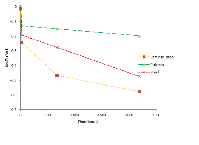
The data from fomite recovery experiments in Dr. Charles Gerba’s lab were fit to the different persistent models. The best fit models are shown in Table 2 and Figure 1 .

Table 2 Best-fit models

Organism Fomite Time(hrs) Best fit model
B. anthracis Polyester 0,24,672,2190 Biphasic exponential
B. anthracis Steel 0,24,672,2190 Biphasic exponential
B. anthracis Laminar 0,24,672,2190 Juneja & Mark(2)


Persistence_model_example.png

Figure 1 Best fit models


Persistence excel tool

Any persistent data could be analyzed by using attached excel spreadsheet. Read the instruction manual first and then use the excel tool accordingly.

Spreadsheet Instruction

Persistence Model wiki

References